Introduction

Over the past couple of days, I’ve been spending the majority of my time really learning the theory behind Support Vector Machines (SVMs). I’ve come across many useful resources including the MIT OCW video on the subject and the almighty Wikipedia for learning about concepts like Karush-Kuhn-Tucker Conditions, Wolfe Duality, and more. I would personally recommend checking out all of those links, as the MIT video provides a nice walkthrough for the math of SVMs and the Wikipedia links clarify the inner workings of that math.

Side Note: While the MIT video is a great resource and was really useful in getting a feel for the math, the professor does makes a simplification when applying Lagrange Multipliers. He sets the constraint for the function to be \(y_i(w\cdot x_i + b) - 1 = 0\). Obviously, this isn’t necessarily true for all \(i\) as it is not necessary for all points to be on the margin of the SVM. The constraint is actually the inequality, \(y_i(w\cdot x_i + b) - 1 \geq 0\). That’s the reason KKT (Karush-Kuhn-Tucker) conditions are applied to the problem, and it’s the reason for the constraint, \(\alpha_i \geq 0\).

After developing somewhat of an understanding of the algorithm, my first project was to create an actual implementation of the SVM algorithm. Though it didn’t end up being entirely from scratch as I used CVXOPT to solve the convex optimization problem, the implementation helped me better understand how the algorithm worked and what the pros and cons of using it were. In this post, I hope to walk you through that implementation. Note that this post assumes an understanding of the underlying math behind SVMs. If you feel uncomfortable on that front, I would again recommend checking out the resources linked above.

The Optimization Problem

Anyways, with that out of the way, let’s get into it! For starters, what is the actual problem we’re trying to solve here? Yes, we want to find the “maximum-margin hyperplane” that separates our two classes, but how do we formalize that goal mathematically? Well, we’ve already seen the following optimization problem:

We’ve seen how we can apply KKT to this problem to in turn get the following Lagrangian Function and constraint:

And we’ve seen how, taking the partial derivative of \(L\) with respect to \(w\) and \(b\), and using them in the equation above, can lead us to the following dual representation of the optimization problem

Now this is a very nice way to represent the problem. The only unknowns in the problem are the \(\lambda\)’s and if you solve for the ones that maximize \(L_D\), you get the solution to our optimization problem. Our \(\lambda\)’s can be used to calculate \(b\) and in turn, the decision boundary for our SVM. So now we just pass our optimization problem to the computer and let it solve it, right? Well, there’s actually a little more prepping to do.

CVXOPT Requirements

The thing is, algorithms that solve convex optimization problems like the one we have here¹, often require the problem in a specific format. Specifically, in the case of CVXOPT, it wants convex optimization problems that it can minimize. It also requires the optimization problem to be in the following format:

Now this seems daunting at first, and I admit it seemed confusing to me as well, but upon closer examination, these expressions are actually very straight-forward.

Before we tackle them, however, let’s deal with the glaring issue with our optimization problem. CVXOPT requires that the problem be a minimization problem, whereas our problem is designed to be maximized. This can actually be easily fixed by simply multiplying our Lagrangian function by \(-1\), creating the following optimization problem:

Multiplying by \(-1\) reflects all values of the \(L_D\) function making positive’s negative and negative’s positive, resulting in the function’s global maximum, becoming a global minimum.

Now let’s put our optimization problem in the form above. Let’s start by looking at the \(\frac{1}{2}x^TPx\) term. If you calculate the value of this expression in terms of the individual elements of the relevant matrices, you get the following:

With this, we see that the \(\frac{1}{2}x^TPx\) term represents all of the second-order variables in the function that needs to be minimized (in our case, the Lagrangian function). We also see that \(P\) is the matrix that satisfies the condition that \(\frac{1}{2}\sum_i^m\sum_j^m x_ix_j\cdot P_{ij}\) is equal to the portion of the Lagrangian function with second-order variables. In our specific case, this portion is \(\sum_i^m \sum_j^m \lambda_i \lambda_j y_i y_j (x_i\cdot x_j)\). Note that \(\lambda_i\) and \(\lambda_j\) represent the \(x_i\) and \(x_j\) in our problem as they are the unknowns. Do not get them mixed up with the \(x_i\) and \(x_j\) in our Lagrangian function as those are just the known data points in our problem. Using this, we get the following definition for \(P\)

In a similar fashion, we see that the \(q^Tx\) term represents all of the first-order variables in the Lagrangian function. We derive the following definition for \(q\) in our problem:

The \(Gx \preceq h\) expression is a linear matrix inequality similar to the form of standard linear matrix equations. It represents any inequality constraints in the optimization problem. In our case, these constraints are \(\lambda_i \geq 0\) for all \(i\) from \(0\) to \(m\). These constraints can be rewritten as \(-\lambda_i \leq 0\) to use the less than or equal to symbol. That gives us the following matrices for \(G\) and \(h\):

Finally, the \(Ax=b\) expression is your standard linear matrix equation and it represents any equality constraints in the optimization problem. In our case, we have a single equation, \(\sum_i^m \lambda_i yi = 0\). With that constraint, we get the following matrices for \(A\) and \(b\):

With matrices for \(P\), \(q\), \(G\), \(h\), \(A\), and \(b\), and a minimizable optimization problem, we are now ready to computationally solve our SVM problem.

The Code - Linear SVM

We’ll start off by importing our relevant modules and creating a basic class for our SVM:

import numpy as np
import matplotlib.pyplot as plt
import seaborn as sns
from cvxopt import matrix, solvers

class SVM:
	def __init__(self):
		pass
	
	def fit(self, X, y):
		pass
	
	def predict(self, u):
		pass
	
	def plot(self):
		pass

Here we’ve created the functions fit(self, X, y), predict(self, u), and plot(self). The fit function will be used to set lambdas and b to the appropriate values for the data set, the predict function will return the predicted class of a given data point, and the plot function will create a visual plot of the data set and the SVM.

The Fit Function

Let’s start by implementing the fit function. First we need to calculate our \(P\), \(q\), \(G\), \(h\), \(A\), and \(b\) matrices:

def fit(self, X, y):
	self.X = X
	self.y = y
	self.m = X.shape[0]
	P = np.empty((self.m, self.m))
	for i in range(self.m):
		for j in range(self.m):
			P[i, j] = y[i]*y[j]*np.dot(X[i], X[j])
	q = -np.ones((self.m, 1))
	G = -np.eye(self.m)
	h = np.zeros((self.m, 1))
	A = y.reshape((1, self.m))
	b = np.zeros((1, 1))

With this, we have all our matrices initialized with self.m set to the amount of data points in X. Note that np.eye(m) gives you an \(m\times m\) matrix with \(1\)’s down the diagonal (also called the \(m\times m\) identity matrix). That way -np.eye(self.m) returns the matrix we want for G.

Now, with the matrices set, we need to convert them to the CVXOPT module’s matrices as the module only reads those objects, and can’t read numpy matrices. This is easy to do as you can convert a numpy matrix to a CVXOPT matrix by doing matrix(numpy_matrix):

def fit(self, X, y):
	...
	P = matrix(P)
	q = matrix(q)
	G = matrix(G)
	h = matrix(h)
	A = matrix(A.astype('double'))
	b = matrix(b)

We modify A to be a matrix with type ‘double’ because it initially contains integers from the y matrix, whereas CVXOPT requires numbers in the form of doubles. The rest of the matrices contain doubles by default, and therefore, don’t require that conversion.

With all the conversions done, we simply need to pass the matrices to CVXOPT to solve the optimization problem. We’ll specifically use the function solvers.qp(P, q, G, h, A, b)

def fit(self, X, y):
	...
	sol = solvers.qp(P, q, G, h, A, b)
	self.lambdas = np.array(sol['x']).reshape(self.m)

Now that we have the lambdas, we need to calculate \(b\). This is done by multiplying both sides of the constraint that support vectors have by \(y_{SV}\) and solving for \(b\):

Plugging in \(w=\sum_i^m \lambda_i y_i x_i\), we get the following:

Now we just need to find a data point that’s a support vector, and we can use it to calculate \(b\). This can be done by using a property of the \(\lambda\)’s. In KKT, the \(\lambda\) multipliers for inequality constraints are only positive if they constrain the optimization problem or in other words, affect the location of the minimum. This makes sense as constraints that don’t constrain the optimization problem, don’t need to be considered and can therefore be nullified by setting their \(\lambda\) multiplier to 0. For a better explanation, I’d recommend reading this paper. In the context of our problem, the constraints that constrain the optimization problem are the ones generated by support vectors. Based on this, a data point with a respective \(\lambda\) that’s greater than 0 will be a support vector.

For our program, we will actually require the \(\lambda\) to be greater than \(10^{-4}\). This is because CVXOPT doesn’t set any \(\lambda\) to \(0\), but rather gets them very close (like \(10^{-8}\)). By requiring the multiplier to be “sufficiently” greater than \(0\), we ensure that non-support vectors aren’t selected.

def fit(self, X, y):
	...
	SV = np.where(self.lambdas > 1e-4)[0][0]
	self.b = y[SV] - sum(self.lambdas * y * np.dot(X, X[SV].T))

And with that, we now have a support vector machine fit to the data set. Now we just need to implement the predict and plot functions.

The Predict Function

This one is fairly straight forward. We’ll use the inequality for the decision boundary and use \(w=\sum_i^m \lambda_i y_i x_i\) to put it in terms of \(\lambda\). Note that in the following inequality \(u\) represents the data point whose class we’re trying to predict.

Our SVM will predict a class of \(1\) if the above inequality is true and \(-1\) otherwise:

def predict(self, u):
	if self.b + sum(self.lambdas * self.y * np.dot(self.X, u.T)) >= 0:
		return 1
	else:
		return -1

The Plot Function

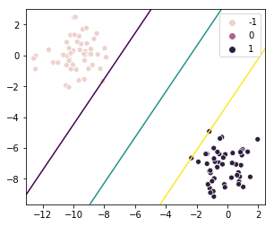
Finally, for the plot function, we will simply plot a contour plot of \(b+\sum_i^m \lambda_i y_i (x_i \cdot u)\) from above and draw the levels where that expression is equal to \(1\), \(0\), or \(-1\). This will give us a plot of the decision boundary and the margins for both classes.

def plot(self):
	x_min = min(self.X[:, 0]) - 0.5
	x_max = max(self.X[:, 0]) + 0.5
	y_min = min(self.X[:, 1]) - 0.5
	y_max = max(self.X[:, 1]) + 0.5
	step = 0.02
	xx, yy = np.meshgrid(np.arange(x_min, x_max, step), np.arange(y_min, y_max, step))
	d = np.concatenate((xx.ravel().reshape(-1, 1), yy.ravel().reshape(-1, 1)), axis=1)

	Z = self.b + np.sum(self.lambdas * self.y * np.dot(self.X, d.T), axis=0)
	Z = Z.reshape(xx.shape)

	fig, ax = plt.subplots()
	sns.scatterplot(x=self.X[:, 0], y=self.X[:, 1], hue=self.y, ax=ax)
	ax.contour(xx, yy, Z, levels=[-1, 0, 1])
	plt.show()

I won’t explain this code as it’s not relevant to SVM’s, but if you find it confusing, I would look into the documentation for MatPlotLib and Seaborn and information on contour plots/scatter plots in those modules.

Let’s Test It

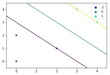
Now that we have a complete SVM class, we just need to generate some training data and pass it to the SVM:

X = np.array([[0, 2], [0, 0], [2, 1], [3, 4], [4, 3]])
y = np.array([-1, -1, -1, 1, 1])

svm = SVM()
svm.fit(X, y)
svm.plot()

This gives us the following plot:

Non-linear SVM using Kernels

So we can separate linearly separable data with a large margin, linear decision boundary. What about cases where the data isn’t linearly separable? Typically, we would add more features to transform the data in a way that allows it to be linearly separated. For example, let’s say we define a function \(\phi\) to create the new data like so:

This may make our data linearly separable in many cases, and we could stop here and use our SVM on this new data. The issue with that is that applying the \(\phi\) function on all the data points is a horribly inefficient operation. For more complex transformations with more features to start off with and more new features to create, this approach ceases to be even remotely reasonable.

Thankfully, SVM’s allow for an alternative way to approach this. One of the reasons SVM’s are so powerful is that they only depend on the dot product of data points (You can check this for yourself. Look at the optimization problem and the decision boundary we’ve used above). The value of the individual data points aren’t required. In the context of the \(\phi\) function, this means we only need to know \(\phi(\vec{x}) \cdot \phi(\vec{y})\) and not the value of any individual \(\phi(\vec{x})\). This dot product of two transformed vectors is what’s called a kernel.

One example of a kernel is the polynomial kernel. It has the following definition:

If we look at the case where \(p=2\) and assume we’re dealing with two-dimensional vectors, we get the following \(\phi\) function:

For higher values of \(p\), the kernel can come from even more features. This grants us the benefit of being able to create a very complex feature space out of our data set without having the drawback of computing expensive transformation functions.

To start implementing this in our code, we need to define a kernel function. For our polynomial kernel, we’ll be using \(p=3\):

def kernel(name, x, y):
	if name == 'linear':
		return np.dot(x, y.T)
	if name == 'poly':
		return (1 + np.dot(x, y.T)) ** 3

Now, we simply need to let the fit function take kernel_name as a parameter and then replace all dot products between two data points with the kernel of them:

def fit(self, X, y, kernel_name='linear'):
	...
	self.kernel_name = kernel_name
	...
	for i in range(self.m):
		for j in range(self.m):
			P[i, j] = y[i]*y[j]*kernel(kernel_name, X[i], X[j])
	...
	self.b = y[SV] - sum(self.lambdas * y * kernel(kernel_name, X, X[SV]))

def predict(self, u):
	if self.b + sum(self.lambdas * self.y * kernel(self.kernel_name, self.X, u)) >= 0:
    ...

def plot(self):
	...
	Z = self.b + np.sum(self.lambdas.reshape((self.m, 1)) * self.y.reshape((self.m, 1)) * kernel(self.kernel_name, self.X, d), axis=0)
	...

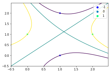
We can test this modified SVM class on a non-linearly separable data set:

X_2 = np.array([[1, 0], [0, 1], [2, 1], [1, 2]])
y_2 = np.array([-1, 1, 1, -1])
svm.fit(X_2, y_2, kernel_name='poly')
svm.plot()

This produces the following plot. We have separated the non-linearly separable data set!

Conclusion

Well that took a lot longer than I expected… What was supposed to be a post of similar length to my first one ended up being almost 3 times as long. Anyways, I hope you got something out of this. I’ll leave a link to the full code below and I encourage you to play around with it. Try out a different kernel, an interesting data set, or a higher dimensional feature space.

As before, I’m sure I’ve made at least a few mistakes in this long post, so if you notice anything that’s off or have any suggestions, please leave a comment below.

Full Code: https://github.com/mbhaskar1/mbhaskar1.github.io/blob/master/code_examples/svm.py

¹ The proof that SVM optimization problems are convex is complex, but it’s a commonly known fact about them and is one of the primary reasons they’re so powerful