Lagrangian Multipliers is a concept commonly taught in Calculus III classes. It’s an amazing mathematical tool that allows you to find the local extrema of any function under a constraint. While it is an incredibly useful tool to have in a mathemetician’s toolkit, in my experience, very few students actually understand how it works. Yes, you set the gradient of the function you’re optimizing equal to some multiplier times the gradient of your constraint, and solving the resulting system gives you the local extrema. But why does that work? In this post, I hope to provide some intuition to answer that question.

Note: This post assumes knowledge of basic concepts of multivariable calculus such as partial derivatives, gradients, etc.

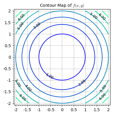
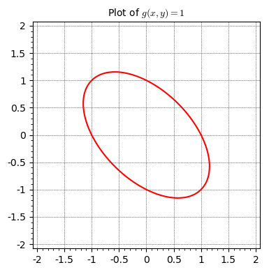
So let’s get started. For the purposes of this post, we’ll be solving a very specific problem. We’ll be trying to find the extrema of the function \(f(x, y)=x^2+y^2\) given the constraint \(g(x, y)=x^2+y^2+xy=1\). Let’s graph both of these functions:

We’ll now proceed by analyzing various properties of either graph at various points. Specifically, we’ll be looking at the gradient of function \(f\) starting at the point \(P_1=(0, 1)\):

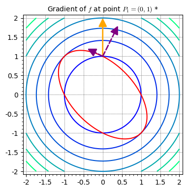
In the above graph, I’ve drawn the gradient vector in orange and then split it into two components, one tangent to the constraint function, and one normal to it. Now, using the definition of a gradient as pointing in the direction of steepest ascent and having a magnitude equal to the “slope” in that direction, we can come to many important conclusions about the point \(P_1\). For example, since the component of the gradient tangent to the constraint function points to the left, we know that as we move a small distance to the left on the constraint function, the value of \(f\) will increase. Similarly, we also know that as we move a small distance to the right on the constraint function, the value of \(f\) will decrease. Combining these two statements, we can say with certainty that the point \((0, 1)\) is not a local extrema for the function \(f\) given our constraint function.

This is analagous to the derivative of a function being negative. The value of the function increases as you decrease the value of the input (move to the left), and just as in the case above, that point can’t be a local extrema.

Now we’re going to look at the point \(P_2=(-1, 1)\):

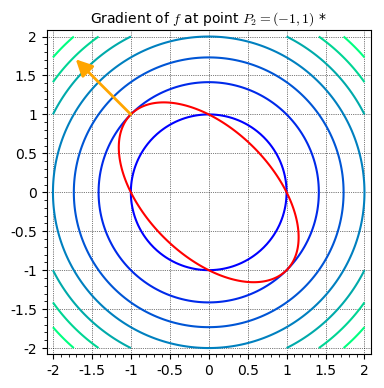
In this case, the gradient vector is perpendicular to the constraint function, and as a result, there is no component tangent to it. If we move a very small distance to the left or right along the constraint function, there will be no change in the function \(f\). As such, the point \(P_2\) can be considered a critical point which can be a local extrema.

This is analagous to the derivative of a function being zero. Small changes in the input of the function cause almost no change in the value of the function, and that particular input can be a local extrema of the function.

With the comparison of these two points, it becomes clear that the key to finding local extrema in constrained optimization problems like this is to find points where the gradient of the function that needs to be optimized, \(f\), is perpendicular to the constraint function, \(g=k\). Just as you set the derivative equal to \(0\) to find the local extrema of a single-variable function, you set the component of the gradient tangent to the constraint function equal to \(0\) to find the local extrema of the constrained multi-variable function.

Now, to represent the goal of finding points where the gradient vector is perpendicular to the constraint function in a solvable form, we need some vector that is always perpendicular to the constraint function. If both vectors have the same direction, we know the gradient vector is perpendicular. It turns out that the gradient of the function \(g\) actually serves as this vector. This is because of the concept in Calculus III that the gradient of a function along a level curve on that function is always perpendicular to that curve. Since our constraint function is in the form \(g(x, y) = k\), it is a level curve of the function \(g\) and therefore, the gradient of \(g\) will be perpendicular to the constraint function.

Knowing all this, we can now just set the gradient of \(f\) equal to some multiple of the gradient of \(g\), setting them to have the same direction:

And there we have the fundamental equation of Lagrangian Multipliers!

I hope that this post made Lagrangian Multipliers make a bit more sense. This is my first post, so I’m sure I’ve made some mistakes here and there, and I’d certainly appreciate any suggestions or improvements.

To keep from leaving things incomplete, I’ll end this by showing the solution to the problem introduced at the beginning of the post.

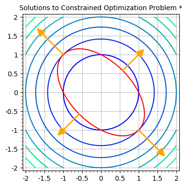
The function \(f\) constrained by \(g=1\) has local minima at points \(\left(-\frac{\sqrt3}{3}, -\frac{\sqrt3}{3}\right)\) and \(\left(\frac{\sqrt3}{3}, \frac{\sqrt3}{3}\right)\), and local maxima at points \((-1, 1)\) and \((1, -1)\).

* The gradient vectors in the graphs in this post have been scaled down to fit in the image