Over the past year, I’ve developed a strong interest in the research area of Algorithmic Game Theory, specifically areas concerned with computational decision making. In learning about topics from this area, I have been working through a very large body of literature. Through this series of “Paper Walkthroughs,” I hope to deepen my understanding of some papers that interest me and to potentially produce some useful content that can be of help to others.

In this specific Paper Walkthrough, I will be conducting a very thorough look at the paper “Learning Equilibria of Simulation Based Games” by Enrique Areyan Viqueria, Cyrus Cousins, Eli Upfal, and Amy Greenwald [1]. I came across this paper after watching a talk on the paper by Dr. Greenwald on YouTube. I feel the problem it tackles is a very practical one with many important real-world applications, and the work also closely aligns with my own research interests. Before I begin discussing the paper, below are some prerequisites that I will assume are met by any reader:

Prerequisites

• A basic understanding of Game Theory concepts (Normal-form games, pure and mixed strategy sets, regret, Nash equilibriums, ϵ-Nash equilibriums, etc.)
• Solid grasp of introductory probability / statistics and introductory calculus
• Familiarity with the notation used in this paper (Read section 2.1)

With that out of the way, let’s get into the paper!

Introduction

So what exactly are “simulation-based games,” and why are they important? In Game Theory, we often concern ourself with games that can be represented in “analytic form,” or as a normal-form game. For example, the Battle of the Sexes game can be represented as a normal-form game:

Battle of the Sexes Game in Normal Form Representation

For those unfamiliar with the Battle of the Sexes game, it models a scenario where a couple is deciding where to go on a day out. They both definitely want to spend time together, but one person would prefer to go to a boxing match, whereas the other would prefer to go shopping. Now suppose that instead of choosing between boxing and shopping, the couple was choosing between two restaurants. Both restaurants have a chef that serves a random meal-of-the-day from a hidden list of a variety of dishes they have learned to cook in their culinary careers. Here, the utility of a person going to one of the restaurants depends on what dish happens to be served on that day. In this case, the normal-form representation of this game would look as follows:

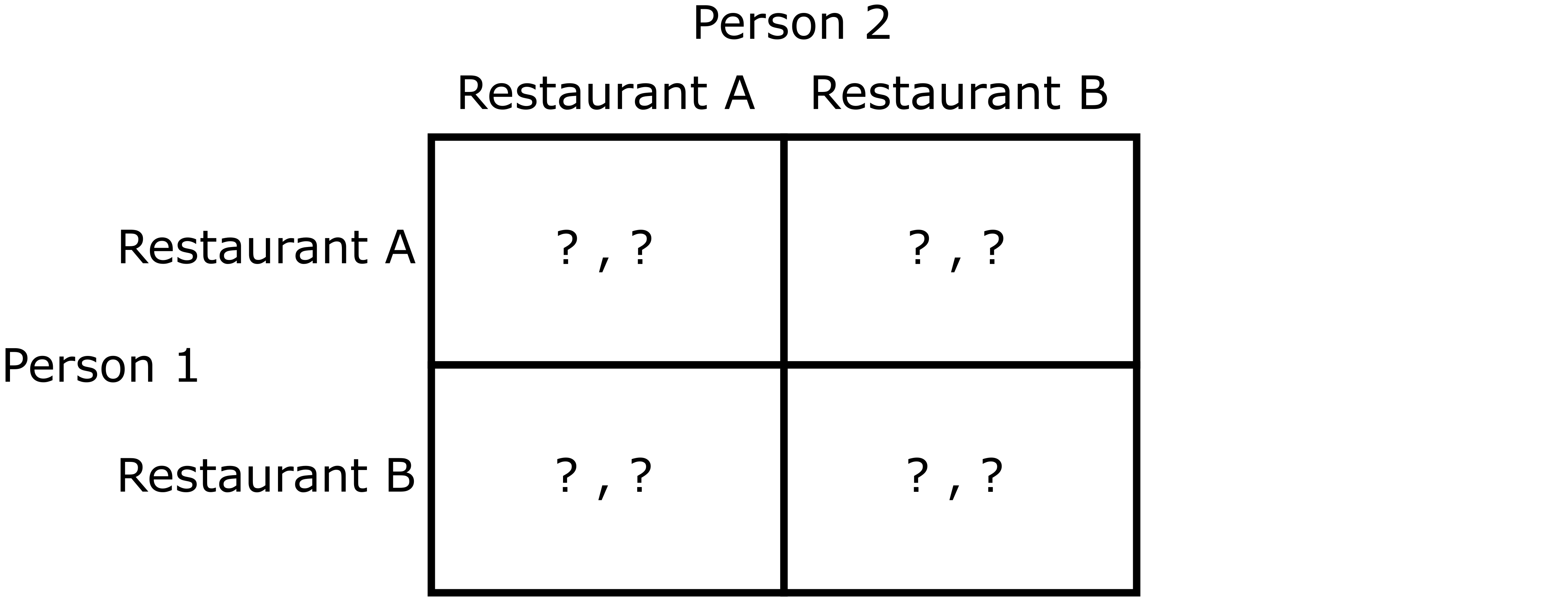Modified Battle of the Sexes Game

Since the distribution through which the chef chooses the meal-of-the-day is unknown, the expected utility for each pure strategy profile cannot be known with absolute precision. To get around this, the couple may sample utilities from each of the possible scenarios, and then approximate each of the expected utilities by the sample average of the respective sampled utilities. Such games where sample utilities are generated to approximate true expected utilities are what this paper calls “simulation-based games.”

Given the chaotic and unpredictable nature of the world we live in, it seems very reasonable that many important decision-making scenarios can be modeled by simulation-based games. We often don’t know the true expected utility of certain actions being taken, but we estimate those utilities through previously recorded data or active sampling. With the notion of simulation-based games in place, several questions come about. How well do simulation-based games approximate the actual underlying games. We imagine that larger sample sizes will result in better approximations, but how good are those approximations with respect to the sample size? Once we have an approximation of some game, we will likely try to find equilibriums using the approximation. In what sense and to what extent do these equilibriums approximate the equilibriums of the true game? Finally, what approach should we use to sample utilities? Should we sample all scenarios or focus our efforts on particular ones? These questions are the focus of the paper we’re looking at today and will be discussed over the course of this Paper Walkthrough.

Formalized Game Structures

Above, we have provided a basic intuition for what a simulation-based game is. In this section, we define a few formal structures, as they have been defined in the paper, that we will use to model simulation-based games. To begin, we introduce the concept of a Conditional Normal-Form Game.

A conditional normal-form game \(\Gamma_\mathcal{X} = \langle \mathcal{X}, P, \{S_p \,\vert \, p\in P\}, u(\cdot, \cdot)\rangle\) consists of a set of conditions \(\mathcal{X}\), a set of agents \(P\), with pure strategy set \(S_p\) available to each agent \(p\), and a vector-valued conditional utility function \(u: S\times \mathcal{X}\mapsto \mathbb{R}^{\vert P\vert}\). In the case of our Modified Battle of the Sexes game from above, a condition would be the meals-of-the-day chosen by each of the two chefs on some particular day. The set of conditions \(\mathcal{X}\) would be the set of all unique pairs of meals-of-the-day that could be chosen by the two chefs. The set of agents \(P\) would contain Person 1 and Person 2. The sets \(S_1\) and \(S_2\), corresponding to Person 1 and Person 2, respectively, would both contain Restaurant A and Restaurant B, representing the pure strategies available to both people in the couple. Finally, the utility function \(u\) would map any pure strategy chosen by the couple, together with a condition, to the resulting utilities experienced by each person.

The problem with the conditional normal-form game is that it doesn’t have any obvious solution concepts. This is because it doesn’t contain information about the liklihood of each condition occurring. To resolve this, we introduce the Expected Normal-Form Game.

Given a conditional normal-form game \(\Gamma_{\mathcal{X}}=\langle \mathcal{X}, P, \{S_p \,\vert \, p\in P\}, u(\cdot, \cdot)\rangle\) and a distribution \(\mathscr{D}\) over \(\mathcal{X}\), we define the expected utility function \(u:S\to \mathbb{R}^{\vert P \vert}\) by \(u(s; \mathscr{D}) = \mathbb{E}_{x\sim \mathscr{D}}[u(s,x)]\), and the corresponding expected normal-form game as \(\Gamma_{\mathscr{D}}=\langle P, \{S_p\,\vert\, p\in P\}, u(\cdot; \mathscr{D})\rangle\). Notice that an expected normal-form game is just a standard normal-form game, and as a result, all the associated solution concepts such as Nash Equilibrium, \(\epsilon\)-Nash Equilibrium, and Correlated Equilibrium apply to it.

This, however leads to another problem. We often don’t have direct access to the distribution \(\mathscr{D}\). For example, in the Modified Battle of the Sexes game, we neither know all the meals that each of the chefs are choosing from, nor the probabilities of them choosing any particular meal. In such situations, we are unable to get the expected utility function, and as a result, we aren’t able to fully define an expected normal-form game. In many such cases, however, we do have indirect access to the distribution through sampling, and can use this access to approximate the expected utility function. This leads to our final game structure: the Empirical Normal-Form Game.

Given a conditional normal-form game \(\Gamma_{\mathcal{X}}\) and a distribution \(\mathscr{D}\) over \(\mathcal{X}\) from which we draw samples \(X=(x_1, \dots, x_m)\sim \mathscr{D}^m\), we define the empirical utility function \(\hat{u}:S\mapsto \mathbb{R}^{\vert P\vert}\) by \(\hat{u}(s; X) = \frac{1}{m}\sum_{j=1}^m u(s, x_j)\), and the corresponding empirical normal-form game as \(\hat{\Gamma}_X=\langle P, \{S_p\,\vert\,p\in P\}, \hat{u}(\cdot;X)\rangle\). Notice that the empirical utility function uses the sample \(X\) to approximate the expected utility function resulting from the same distribution and game. In this sense, the empirical normal-form game can be seen as an approximation of the corresponding expected normal-form game. Like the expected normal-form game, this game structure is also a standard normal-form game and can be solved for various standard solution concepts. This is the game structure we will use to represent simulation-based games.

Designing a Metric Function

With a formal game structure in place, we can now begin to work towards answering some of the questions from earlier. The question that’s the greatest focus of this paper is, for any given number of samples, how closely does an empirical normal-form game approximate its corresponding expected normal-form game. In order to begin to answer this question, we need some way of measuring the “closeness” of two normal-form games differing only in their utility functions. In other words, we need a metric function.

Consider the metric function \(d_\infty\) defined by \(d_\infty(\Gamma, \Gamma'):=\vert\vert\Gamma - \Gamma'\vert\vert_\infty:=\sup_{p\in P, s\in S}\vert u_p(s) - u'_p(s)\vert\). Though the paper only defines the infinity norm, creating an explicit metric function makes it clear we are trying to measure the “closeness” of any two games. In this case, the metric function \(d_\infty\) measures the closeness of the utility functions of two games by measuring the least upper bound on the difference between corresponding utilities in both games. Though it’s not immediately obvious, this least upper bound also applies to utilities for mixed strategies, even though it doesn’t directly consider them. This is proven below in a manner similar to the proof of Lemma 2.4 from the paper.

Lemma 2.4: For any two normal-form games, \(\Gamma\) and \(\Gamma'\), differing only in their utility functions, the least upper bound on the difference between corresponding utilities, including those for mixed strategies, is \(d_\infty(\Gamma, \Gamma')\).

Proof: Let \(\Gamma, \Gamma'\) be arbitrary games that differ only in their utility functions \(u\) and \(u'\). Let \(P\) be the agents involved in both games, and let \(S\) denote the pure strategy profile space for both games. For any agent \(p\) and mixed strategy profile \(\tau\in S^\diamond\), we have \(u_p(\tau)=\sum_{s\in S} \tau(s)u_p(s)\), where \(\tau(s) = \prod_{p'\in P} \tau_{p'}(s_{p'})\), and \(\tau_{p'}(s_{p'})\) is the probability of agent \(p'\) choosing pure strategy \(s_{p'}\). Notice that by its definition, we have that \(\tau(s)\geq 0\) for all \(s\in S\) and that \(\sum_{s\in S}\tau(s)=1\). For all \(p\in P\) and \(\tau\in S^\diamond\), we then have

Since \(\vert u_p(\tau) - u'_p(\tau)\vert\leq d_\infty(\Gamma, \Gamma')\) for all \(p\in P\) and \(\tau\in S^\diamond\), we have that

Therefore, we have shown that \(d_\infty\) does measure the least upper bound on the difference between any corresponding utilities, including those for mixed strategies, of two games differing only in their utility functions.

Given the above Lemma, it seems reasonable to use \(d_\infty\) as a measure of closeness between similarly structured games. The smaller \(d_\infty(\Gamma, \Gamma')\) is, the closer the utility functions of the two games are guaranteed to be. If \(d_\infty(\Gamma, \Gamma')=0\), then \(\Gamma\) and \(\Gamma'\) are identical. What is not immediately so clear is why “closeness” under this metric is desireable. In our specific context, we aim to have an empirical normal-form game be close to its corresponding expected normal-form game, in hopes that solving the empirical normal-form game will approximate the solutions of the expected normal-form game. Through Theorem 2.6 from the paper, we will see that \(d_\infty\) is an appropriate metric for this goal.

Theorem 2.6 (Approximability of Equilibria): If two normal-form games, \(\Gamma\) and \(\Gamma'\), satisfy \(d_\infty(\Gamma, \Gamma')\leq \epsilon\), then:

Proof: This proof follows the exact reasoning used for the corresponding proof in the paper. Let \(\Gamma\) and \(\Gamma'\) be normal-form games with agents \(P\), pure strategy profile space \(S\), and utility functions \(u\) and \(u'\), respectively, and suppose that \(d_\infty(\Gamma, \Gamma')\leq \epsilon\). Since all pure Nash equilibria are also mixed Nash equilibria, and all pure \(\epsilon\)-Nash equilibria are also mixed \(\epsilon\)-Nash equilibria, it is only necessary to prove statement (2). This will be done by first showing that \(E^\diamond_\gamma(\Gamma)\subseteq E_{2\epsilon + \gamma}^\diamond(\Gamma')\) for all \(\gamma\geq 0\).

Let \(\gamma\geq 0\) and suppose that \(s\in E^\diamond_{\gamma}(\Gamma)\). Fix an agent \(p\), and define \(T_{p, s}^\diamond:= \{\tau\in S^\diamond\,\vert\, \tau_q = s_q,\, \forall q\neq p\}\), representing the set of all mixed strategy profiles in which the strategies of all agents \(q\neq p\) match those in \(s\). Let \(s^* \in \textrm{argmax}_{\tau\in T_{p, s}^\diamond}u_p(\tau)\) and \(s'^* \in \textrm{argmax}_{\tau\in T_{p, s}^\diamond}u'_p(\tau)\). By the definition of regret, we have

By Lemma 2.4 and the fact that \(d_\infty(\Gamma, \Gamma')\leq \epsilon\), we have that \(\vert u_p(s'^*)-u'_p(s'^*)\vert \leq \epsilon\) and that \(\vert u_p(s) - u'_p(s)\vert \leq \epsilon\). Through basic algebraic manipulation, this implies that \(u'_p(s'^*)\leq u_p(s'^*) + \epsilon\) and that \(u'_p(s)\geq u_p(s) - \epsilon\), which together imply that

But since \(s^*\in \textrm{argmax}_{\tau\in T_{p, s}^\diamond}u_p(\tau)\), we have that \(u_p(\tau)\leq u_p(s^*)\) for all \(\tau\in T_{p, s}\). Since \(s'^*\in T_{p, s}\), we have that \(u_p(s'^*)\leq u_p(s^*)\), implying that

Finally, since \(s\in E^\diamond_{\gamma}(\Gamma)\), we have \(\textrm{Reg}_p(\Gamma, s)\leq \gamma\). Since \(s^*\in T_{p, s}\), by the definition of regret, we have \(u_p(s^*) - u_p(s)\leq \textrm{Reg}_p(\Gamma, s)\leq \gamma\). With basic algebraic manipulation, this gives us \(u_p(s)\geq u_p(s^*) - \gamma\), which implies that

Since \(p\) was arbitrary, we have that \(\textrm{Reg}_p(\Gamma', s)\leq 2\epsilon + \gamma\) for all \(p\in P\), and therefore, we have shown that \(s\in E_{2\epsilon + \gamma}^\diamond(\Gamma')\). Since \(s\) and \(\gamma\) were arbitrary, we have shown that \(E^\diamond_\gamma(\Gamma)\subseteq E_{2\epsilon + \gamma}^\diamond(\Gamma')\) for all \(\gamma\geq 0\). Note that since \(d_\infty(\Gamma, \Gamma') = d_\infty(\Gamma', \Gamma)\), the symbols \(\Gamma\) and \(\Gamma'\) can be swapped in the above reasoning to also get us that \(E^\diamond_{\gamma'}(\Gamma')\subseteq E_{2\epsilon + \gamma'}^\diamond(\Gamma)\) for all \(\gamma'\geq 0\). Setting \(\gamma=0\) gives us \(E^\diamond(\Gamma)\subseteq E_{2\epsilon}^\diamond(\Gamma')\), and setting \(\gamma'=2\epsilon\) gives us \(E^\diamond_{2\epsilon}(\Gamma')\subseteq E_{4\epsilon}^\diamond(\Gamma)\). Therefore, we have succeeded in showing that

Since \(\Gamma\) and \(\Gamma'\) were arbitrary, we are done.

The above Theorem tells us that if we have an expected normal-form game \(\Gamma_\mathscr{D}\) that we approximate using an empirical normal-form game \(\Gamma_X\) satisfying \(d_\infty(\Gamma_X, \Gamma_\mathscr{D})\leq \epsilon\), then any \(2\epsilon\)-Nash equilibria of \(\Gamma_X\) will be at least a \(4\epsilon\)-Nash equilibrium of \(\Gamma_\mathscr{D}\), and furthermore, all the true Nash equilibria of \(\Gamma_\mathscr{D}\) will be contained in the set of \(2\epsilon\)-Nash equilibria of \(\Gamma_X\). As a result of this, we see that under the metric \(d_\infty\), closeness between an empirical normal-form game and its corresponding expected normal-form game is desireable, and hence, the metric \(d_\infty\) is an appropriate metric to analyze when considering our questions.

Probably Approximately Correct Framework

Having settled on a metric function to measure the closeness of similarly structured games, we can now restate our earlier question. For a given sample \(X\sim \mathscr{D}^m\), how closely – using \(d_\infty\) as the metric for closeness – does an empirical normal-form game \(\Gamma_X\) approximate its corresponding expected normal-form game \(\Gamma_\mathscr{D}\)? Now, we are interested in this question in contexts where the only access to \(\mathscr{D}\) is through sampling. As a result, a concrete value for \(d_\infty(\Gamma_X, \Gamma_\mathscr{D})\), or even an upper bound on it, cannot be found. For example, even if a certain utility is 10 for 1000 sampled conditions, it is still possible that those sample conditions were all outliers, and the true expected value of that utility could be any other value. Though we can’t find such upper bounds that always apply, we may be able to find upper bounds that hold with high probability. This kind of approach is known as Probably Approximately Correct (PAC) Learning.

Formally, after applying the PAC approach to our question, for any given error-rate \(\delta\in (0, 1)\), we aim to find a corresponding \(\epsilon>0\), with smaller \(\epsilon\) being preferred to larger ones, such that

This is a productive direction to take our initial question, as it aims not only to find strong bounds on \(d_\infty(\Gamma_X, \Gamma_\mathscr{D})\) that hold with high probability but also to use Theorem 2.6 from above to make guarantees about the strength of the epsilon-equilibria of \(\Gamma_X\) when applied to \(\Gamma_\mathscr{D}\). In Part 2 of this Paper Walkthrough, we will conduct an in-depth look into the methods used by the paper for finding small \(\epsilon\) and the theory behind each approach.

References

[1] Viqueira, Enrique Areyan, et al. “Learning Equilibria of Simulation-Based Games.” ArXiv:1905.13379 [Cs], May 2019. arXiv.org, http://arxiv.org/abs/1905.13379.